Web Prolog Tutorial
Introduction
Web Prolog is Prolog with two things added: a network and a process model. The simplest nodes just speak HTTP and evaluate logical queries on demand; the richer ones also speak WebSocket and host Erlang-style actors, each with its own mailbox.
The same Prolog predicates work whether the other side of the conversation is a function on this node, an actor across the room, or a service on another continent — remote calls that read like local ones, distribution that disappears into the language.
Web Prolog nodes do not all have to do everything. A small hierarchy of profiles — ISOBASE, ISOTOPE, ACTOR — lets a node advertise exactly how much of the system it implements, and this tutorial walks up that hierarchy: pure relational queries first, then session state, then actors, then the higher-level patterns (server behaviours, statecharts) that build on actors. You can stop at any level; each one is a coherent way to use the system.
Local ISOBASE programming
ISOBASE programming starts with ordinary, side-effect-free Prolog queries.
These examples use local predicates hosted by the current node and are safe
to run through the stateless /call API.
If you are reading this inside the portal, use the terminal to the right.
Queries must end with a full stop. If a query has more than one answer,
press ; or the space bar for more, or use the green Next button.
API checkbox at the bottom of the Logger, you can
watch the HTTP traffic generated by your queries.
append/3 in two modes
Prolog is a relational language. The same predicate can often be used in
more than one direction. First, use append/3 in the ordinary
way to join two lists:
?- append([a],[b,c],Xs).
Now run the same predicate backwards and let Prolog split a list in all possible ways:
?- append(Xs,Ys,[a,b,c]).
This second query has several answers. Again, press ; or the space bar for more, or use the green Next button.
A small family program
This node hosts some shared Prolog code. The small family program below is part of that shared database, so you can query it directly.
ancestor_descendant(X, Y) :-
    parent_child(X, Y).
ancestor_descendant(X, Z) :-
    parent_child(X, Y),
    ancestor_descendant(Y, Z).

parent_child(X, Y) :-
    mother_child(X, Y).
parent_child(X, Y) :-
    father_child(X, Y).

mother_child(trude, sally).

father_child(tom, sally).
father_child(tom, erica).
father_child(mike, tom).
Ask for Mike's descendants:
?- ancestor_descendant(mike, Who).
Stateless API limitations
ISOBASE requests are independent: the server returns an answer or reaches its request limit, then forgets the execution context. This deliberately rules out the controls available on persistent ISOTOPE and ACTOR sessions.
That trade-off is useful when each query is self-contained: clients can use ordinary HTTP, requests cannot leave session state behind, and the node can enforce a clear time and resource bound for every call.
No abort
There is no client-side abort operation for a stateless call. This goal runs until n1's request timeout expires (currently two seconds):
?- repeat, fail.
No I/O
Output and input need a persistent conversation with the client, so they are not part of the stateless API. The node rejects this call:
?- writeln(hello).
No dynamic database manipulation
A change made during one stateless request would have no session in which to persist, so dynamic database updates are unavailable as well:
?- assertz(p(1)).
Movie database
Node n1 hosts a movie database. Its facts describe films,
directors, actors, and actresses, and can be queried directly through the
stateless /call API.
Find films by year
?- movie(Film, 2000).
Find co-stars
This query finds pairs of performers who appeared in the same film:
?- actor(Film, First, _), actor(Film, Second, _), First @> Second.
Find directors who also acted
?- actor(_, Person, _), director(_, Person).
Parsing and generating with a DCG
A Definite Clause Grammar (DCG) is a clean Prolog notation for grammars. Load this small one into your session, and you can use it to parse or generate sentences:
s(s(NP,VP)) --> np(NP, Num), vp(VP, Num).

np(NP, Num) --> pn(NP, Num).
np(np(Det,N), Num) --> det(Det, Num), n(N, Num).
np(np(Det,N,PP), Num) --> det(Det, Num), n(N, Num), pp(PP).

vp(vp(V,NP), Num) --> v(V, Num), np(NP, _).
vp(vp(V,NP,PP), Num) --> v(V, Num), np(NP, _), pp(PP).

pp(pp(P,NP)) --> p(P), np(NP, _).

det(det(a), sg) --> [a].
det(det(the), _) --> [the].

pn(pn(john), sg) --> [john].

n(n(man), sg) --> [man].
n(n(men), pl) --> [men].
n(n(telescope), sg) --> [telescope].

v(v(sees), sg) --> [sees].
v(v(see), pl) --> [see].
v(v(saw), _) --> [saw].

p(p(with)) --> [with].
Ask for a parse tree:
?- phrase(s(Tree), [john,saw,a,man,with,a,telescope]).
You can also use the same grammar for generation:
?- forall((between(1,8,N), length(S,N), phrase(s(_),S)), writeln(S)).
Distributed ISOBASE programming
ISOBASE nodes can be composed across HTTP. The simplest form is a remote query that behaves like ordinary Prolog backtracking; the promise form lets you start the remote work first and collect the answer later.
Remote calls with rpc/2-3
Web Prolog nodes can talk to each other. The predicate
rpc/2-3 sends a goal to a remote node identified by a URI,
receives the answers over the stateless /call API, and turns
them back into ordinary Prolog backtracking.
Note that rpc/2-3 talks specifically to the remote node's
stateless /call route. This remains true even if the target
happens to be an ACTOR node. So rpc/2-3 can be used for
remote logical queries, but not for actor-only goals such as
self/1, spawn/1-3, or receive/1-2.
In this deployment, n1 hosts:
human(plato).
human(aristotle).
while n2 hosts:
mortal(Who) :- human(Who).

human(socrates).
human(Who) :-
    rpc('https://n1.elfenbenstornet.se', human(Who)).
From this portal, you can query n2 directly:
?- rpc('https://n2.elfenbenstornet.se', mortal(Who)).
You should get
socrates from n2 itself, followed by
plato and aristotle fetched remotely from
n1.
Remote calls with promises
promise/3-4 starts an asynchronous remote query and returns a
reference. Later, yield/2-3 collects the answer produced by
that remote call.
?- promise('https://n2.elfenbenstornet.se', mortal(Who), Ref).
?- yield($Ref, Answer).
The answer is returned as the same Prolog term format used by the stateless remote call. The promise is useful when the caller has other work to do before it needs the result.
That is essentially all of distributed ISOBASE: synchronous remote calls
via rpc/2-3, plus their asynchronous cousins
promise/3-4 and yield/2-3. Anything more —
session state, side effects, actors that survive between requests —
needs the ISOTOPE or ACTOR profile, which the rest of the tutorial covers.
Local ISOTOPE programming
ISOTOPE adds persistent toplevel sessions to ISOBASE. That makes it possible to keep session-local state, perform I/O, and change the dynamic database while the session is alive.
Reading and writing
hello_world :-
    writeln('Hello World!'),
    sleep(1),
    hello_world.

read_and_write :-
    writeln('Type a term or \'stop\''),
    read(Something),
    (   Something == stop
    ->  true
    ;   writeln(Something),
        read_and_write
    ).
?- hello_world.
?- read_and_write.
Database manipulation
:- dynamic p/1.

assert_and_retract :-
    forall(between(1, 10, X), assert(p(X))),
    forall(retract(p(X)), writeln(X)).

assert_many(Count) :-
    forall(between(1, Count, X), assert(p(X))),
    retractall(p(_)).
?- assert_and_retract.
?- time(assert_many(1_000_000)).
Distributed ISOTOPE programming
Predicate shipping
The three-argument form of rpc/2-3 can also ship temporary
source text with the call. Here mortal/1 is defined only for
the duration of the remote query:
?- rpc('https://n1.elfenbenstornet.se', mortal(Who), [
       load_text("mortal(Who) :- human(Who).")
   ]).
The code passed in load_text/1 is not installed permanently;
it exists only for that remote call.
Distributed proof trees
A defining advantage of logic-based AI is transparency: every conclusion rests on rules and facts, and an explanation can be constructed as a proof object. On the Prolog Web, explanations can survive distribution. If a subgoal is proved on another node, its justification is folded into the same overall proof structure rather than hidden inside an opaque remote call.
A compact meta-interpreter achieves this by treating remote calls as
proof-producing sub-derivations. When the interpreter encounters a remote
goal it ships itself to the remote node via
load_predicates([prove/2]), so the remote node also runs
prove/2 and returns a proof term. Remote contributions are
marked in the result with the @ operator.
n2, which has
the distributed mortal/1 and human/1 definitions
in its shared database.
Load the interpreter into your session:
prove(true, true) :- !.
prove(rpc(URI, A), Proof) :- !,
    prove(rpc(URI, A, []), Proof).
prove(rpc(URI, A, Options), Query@URI/Proof) :- !,
    rpc(URI, prove(A, Query/Proof), [
        load_predicates([prove/2])
      | Options
    ]).
prove((A, B), (ProofA, ProofB)) :- !,
    prove(A, ProofA),
    prove(B, ProofB).
prove(A, A/Proof) :-
    clause(A, B),
    prove(B, Proof).
On n2, the shared database contains:
:- dynamic mortal/1, human/1.

mortal(X) :- human(X).

human(socrates).
human(X) :- rpc('https://n1.elfenbenstornet.se', human(X)).
while n1 hosts:
:- dynamic human/1.

human(plato).
human(aristotle).
Now ask for a proof:
?- prove(mortal(X), Proof).
You should see something like:
Proof = mortal(socrates)/(human(socrates)/true),
X = socrates ;
Proof = mortal(plato)/(human(plato)/(human(plato)@'https://n4.elfenbenstornet.se'/true)),
X = plato ;
Proof = mortal(aristotle)/(human(aristotle)/(human(aristotle)@'https://n4.elfenbenstornet.se'/true)),
X = aristotle.
The first answer is proved entirely on n2. The second and
third are proved by delegating to n1, and the annotation
@'https://n1.elfenbenstornet.se' documents exactly where each
remote step was resolved. The proof term is ordinary Prolog data: it can be
inspected, stored, or rendered into a human-readable explanation.
clause/2 can only inspect predicates
declared dynamic.
Programming with the Semantic Web
The Semantic Web envisions a machine-readable layer over the existing Web, built on shared identifiers (URIs), a triple-based data model (RDF), and a rule layer for inference. Web Prolog overlaps that vision substantially: Prolog is already a rule-based language operating over relational facts. The simplest way to bring the two together is to represent triples as Prolog facts and write the application's public interface as ordinary predicates over them.
RDF triples and rules over them
An RDF triple has the form <subject, predicate, object>. In Web
Prolog we represent each triple as a three-argument fact
rdf/3. The fragment below uses two well-known vocabularies
— FOAF for people and knows-relations, and schema.org for typed
values — and adds one Prolog rule,
known_with_birthdate/3, that joins two triples to answer
"people that someone knows, together with their birthdates":
:- dynamic rdf/3.

rdf('http://example.org/bob#me',
    'http://www.w3.org/1999/02/22-rdf-syntax-ns#type',
    'http://xmlns.com/foaf/0.1/Person').

rdf('http://example.org/bob#me',
    'http://xmlns.com/foaf/0.1/knows',
    'http://example.org/alice#me').

rdf('http://example.org/bob#me',
    'http://xmlns.com/foaf/0.1/knows',
    'http://example.org/charlie#me').

rdf('http://example.org/alice#me',
    'http://schema.org/birthDate',
    literal(type('http://www.w3.org/2001/XMLSchema#date', '1990-07-04'))).

rdf('http://example.org/charlie#me',
    'http://schema.org/birthDate',
    literal(type('http://www.w3.org/2001/XMLSchema#date', '1985-12-23'))).

known_with_birthdate(Me, He, Date) :-
    rdf(Me, 'http://xmlns.com/foaf/0.1/knows', He),
    rdf(He, 'http://schema.org/birthDate', Date).
The URIs are deliberately long because they are real identifiers, not
local names. Two parties using http://xmlns.com/foaf/0.1/knows
are talking about the same relation no matter which Prolog system or
database the data came from. That is the value the Semantic Web adds:
shared meaning through shared identifiers.
With the data and rule loaded, first query the raw triples — who does Bob know?
?- rdf('http://example.org/bob#me',
       'http://xmlns.com/foaf/0.1/knows',
       Who).
Then query through the rule, which joins two triples in one step:
?- known_with_birthdate(Me, He, Date).
This is the essence of one Prolog Web cooperation pattern: RDF is the
interchange format and the storage substrate, but the application's
public interface is named Prolog predicates. Callers do not need to know
which triples were consulted; they ask
known_with_birthdate/3, and the predicate is free to evolve
internally — more clauses, additional joins, cross-vocabulary
mapping — without changing the contract.
The same code can also be hosted by an ISOBASE node and queried from
anywhere with rpc/2-3, exactly like the family program
earlier in the tutorial. RDF provides interoperable identifiers and
shared meaning; Prolog provides an executable, composable, reusable rule
layer on top of them. The Semantic Web and the Prolog Web compose
naturally.
Local ACTOR programming
Web Prolog extends Prolog with Erlang-style message-passing concurrency. An actor is a lightweight isolated process with its own mailbox and its own private Prolog database, identified by a process id called a pid; actors interact only by sending each other messages, never by sharing memory.
The terminal session to the right is itself an actor. We will use it to send messages, inspect the mailbox, spawn other actors, and watch what happens when actors terminate. The examples that follow do not just borrow Erlang's vocabulary — programmed in the Erlang style, actors here behave the way Erlang actors do.
The session is persistent, so run the examples in order — later examples build on bindings and actors created by earlier ones.
The shell's pid
The terminal to the right is running a Web Prolog shell. The core of a shell is a toplevel actor. Start by asking the shell for its process identifier (pid for short):
?- self(Self).
A pid is the address of an actor. If you know a pid, you can send that actor a message.
Sending a message
The shell understands dollar notation: $Self means "use the
most recent value of Self". Send the shell a message:
?- $Self ! hello.
Now receive the oldest matching message from the mailbox:
?- receive({Message -> true}).
You should get Message = hello. If the mailbox is empty,
receive/1 waits until a matching message arrives.
Inspecting the mailbox
flush/0 is a shell utility: it prints every pending message
and never blocks.
?- $Self ! hello, $Self ! goodbye.
?- flush.
This is usually the quickest way to see what is sitting in your mailbox while you are experimenting.
Spawning an actor
An actor is capable of spawning other actors and then talking to them. This node hosts a tiny echo actor:
echo_actor :-
    receive({
        echo(From, Msg) ->
            From ! echo(Msg),
            echo_actor
    }).
Spawn it:
?- spawn(echo_actor, Pid).
Then send it a request. The reply comes back asynchronously to your shell mailbox:
?- self(Self), $Pid ! echo(Self, hi).
?- flush.
Visible actors
Web Prolog supports the predicate actors/1, which binds its
argument to the list of pids of all actors visible from your current
session:
?- actors(Alive).
The first item is the pid of your shell; the echo actor you just spawned should also be in the list.
Linking
By default, a child is linked to its parent. If the parent exits, linked children are terminated too.
?- spawn(spawn(receive({}))).
Now inspect the actors visible from your current session again:
?- actors(Alive).
The inner nonterminating actor does not survive as a new long-lived child because linking ensures that when the outer spawned actor terminates, its child is taken down with it.
Linking is one-way. A child that exits does not kill its parent:
?- spawn((spawn(exit(kill)), receive({})), Pid).
?- actors(Alive).
You should now see one extra live actor: the parent is still there even though its child exited immediately. Clean it up before moving on:
?- exit($Pid, cleanup).
Monitors
If you spawn with monitor(true), the child sends a
down/3 notification when it terminates:
?- spawn(2 > 1, Pid, [monitor(true)]).
The notification lands in the shell mailbox, so inspect it with
flush/0:
?- flush.
The message has the form down(Ref, Pid, Reason). Here the
actor succeeds normally, so the reason should be true.
Explicit monitors
monitor(true) is the simple case. You can also install
monitors explicitly with monitor/2. Each monitor gets its own
reference and therefore its own down/3 message.
?- spawn(sleep(1), Pid),
   monitor(Pid, Ref1),
   monitor(Pid, Ref2),
   sleep(1.2),
   flush.
If you remove the monitor before the child terminates, the
down/3 message never arrives.
?- spawn(sleep(1), Pid),
   monitor(Pid, Ref),
   demonitor(Ref),
   receive({
       down(_, Pid, _) ->
           writeln('Unexpected down message.')
   }, [
       timeout(1.2),
       on_timeout(writeln('No down message arrived.'))
   ]).
monitor(true) on spawn/3. It installs the monitor
atomically with process creation and avoids the race where the child exits
before a later call to monitor/2 has been set up.
Registered names
You can register a pid under a name and use the name instead of the pid.
The inverse, unregister/1, drops the name when you no longer
need it. Here the shell registers itself under the name shell:
?- self(Self), register(shell, Self).
?- shell ! hello.
?- spawn(shell ! goodbye).
?- flush.
Killing an actor
Some actors do not stop on their own. Here we spawn a monitored echo actor,
register it under a name, and then terminate it with exit/2:
?- spawn(echo_actor, Pid, [monitor(true)]),
   register(echo_actor, Pid).
?- whereis(echo_actor, Pid),
   exit(Pid, 'We changed our minds!').
Because the actor was monitored, the mailbox now contains a
down(...) message with the exit reason.
?- flush.
Choosing an exit reason
A monitored actor can stop itself with exit/1. The reason
ends up in the down/3 message:
?- spawn(exit(my_reason), Pid, [monitor(true)]).
?- flush.
Sending to a dead pid is just a no-op, so monitors are the usual way to learn that an actor has gone away.
Selective receive
receive/1 does not have to take the oldest message. It scans
the mailbox for the first message that matches one of its receive clauses
and leaves the others in place. This example insists on handling
hello before goodbye even if
goodbye arrives first.
wait_hello :-
    receive({
        hello ->
            writeln('Got hello.'),
            wait_goodbye
    }).

wait_goodbye :-
    receive({
        goodbye ->
            writeln('Got goodbye.')
    }).
?- self(Self),
   Self ! goodbye,
   Self ! hello,
   wait_hello.
The first receive/1 skips goodbye, consumes
hello, and the second receive/1 then picks up the
deferred message. This selective behavior is one of the core ideas in
Erlang-style message passing.
Multi-clause receive
A receive call can have several clauses. The first matching clause wins, and unmatched messages are left in the mailbox for later.
?- self(Self),
   Self ! goodbye(bob),
   receive({
       hello(Name) ->
           format("Hello, ~w!~n", [Name]) ;
       goodbye(Name) ->
           format("Goodbye, ~w!~n", [Name])
   }).
Guards and timeouts
Receive clauses can also have guards. Here the same pattern is handled in two different ways depending on the number inside the message.
?- self(Self),
   Self ! number(-2),
   receive({
       number(N) if N > 0 ->
           format("Positive number: ~p~n", [N]) ;
       number(N) if N =< 0 ->
           format("Non-positive number: ~p~n", [N])
   }).
If you do not want to wait forever, add a timeout. This waits one second for a matching message and prints a note if nothing shows up.
?- receive({
       person(Name) ->
           format("Hello, ~w!~n", [Name])
   }, [
       timeout(1),
       on_timeout(writeln('No person arrived.'))
   ]).
A small priority queue
This example, borrowed from Fred Hébert's Learn You Some Erlang for Great Good!, uses guards plus zero-timeout receives to sort "important" messages before normal ones. First load the predicates into your current session:
important(Messages) :-
    receive({
        Priority-Message if Priority > 10 ->
            Messages = [Message|MoreMessages],
            important(MoreMessages)
    }, [
        timeout(0),
        on_timeout(normal(Messages))
    ]).

normal(Messages) :-
    receive({
        _-Message ->
            Messages = [Message|MoreMessages],
            normal(MoreMessages)
    }, [
        timeout(0),
        on_timeout(Messages = [])
    ]).
Now send four messages to yourself:
?- self(S),
   S ! 15-high,
   S ! 7-low,
   S ! 1-low,
   S ! 17-high.
Then ask the queue to collect them in priority order:
?- important(Messages).
The result should be Messages = [high,high,low,low]. This
works only because unmatched messages are deferred rather than discarded.
A count server
This actor keeps its state in an argument. Each count(From)
message increments the counter and sends the new count back. A
stop message terminates the server cleanly.
count_actor(Count0) :-
    receive({
        count(From) ->
            Count is Count0 + 1,
            From ! count(Count),
            count_actor(Count) ;
        stop ->
            true
    }).
?- spawn(count_actor(0), Pid, [
       monitor(true)
   ]).
?- self(Self).
?- $Pid ! count($Self).
?- receive({Count -> true}).
?- $Pid ! count($Self), $Pid ! stop.
?- flush.
Because the actor was monitored, the final flush/0 should
show both the updated count and a down(...) message.
A fridge simulation
The following example, also adapted from Fred Hébert's Learn You Some Erlang for Great Good!, simulates a fridge that keeps its state as a list of food items. Messages are used to store food, take food, or terminate the server.
fridge(FoodList0) :-
    receive({
        store(From, Food) ->
            self(Self),
            From ! Self-ok,
            fridge([Food|FoodList0]);
        take(From, Food) ->
            self(Self),
            (   select(Food, FoodList0, FoodList)
            ->  From ! Self-ok(Food),
                fridge(FoodList)
            ;   From ! Self-not_found,
                fridge(FoodList0)
            );
        terminate ->
            true
    }).
?- spawn(fridge([]), Pid, [
       monitor(true)
   ]).
?- self(Me), $Pid ! store(Me, meat), $Pid ! store(Me, cheese).
?- flush.
?- self(Me), $Pid ! take(Me, cheese).
?- flush.
?- $Pid ! terminate.
?- flush.
Hiding the protocol details
Raw message sending works, but it forces the client to remember the protocol. The usual fix is to wrap the protocol in ordinary predicates.
store(Pid, Food, Response) :-
    self(Self),
    Pid ! store(Self, Food),
    receive({
        Pid-Response -> true
    }).

take(Pid, Food, Response) :-
    self(Self),
    Pid ! take(Self, Food),
    receive({
        Pid-Response -> true
    }).
These helpers are available on the node, so you can use them directly:
?- spawn(fridge([]), Pid, [
       monitor(true)
   ]).
?- store($Pid, cheese, Response).
?- take($Pid, cheese, Response).
?- $Pid ! terminate.
?- flush.
This style is easier to read and much easier to reuse. The actor still speaks the same message protocol, but clients no longer need to handle it explicitly.
Actors playing ping-pong
This example is adapted from the official Erlang message-passing guide. Two actors send messages back and forth three times, then finish.
ping(0, Pong_Pid) :-
    Pong_Pid ! finished,
    format('Ping finished.~n',[]).
ping(N, Pong_Pid) :-
    self(Self),
    Pong_Pid ! ping(Self),
    receive({
        pong ->
            format('Ping received pong.~n',[])
    }),
    N1 is N - 1,
    ping(N1, Pong_Pid).

pong :-
    receive({
        finished ->
            format('Pong finished.~n',[]) ;
        ping(Ping_Pid) ->
            format('Pong received ping.~n',[]),
            Ping_Pid ! pong,
            pong
    }).

ping_pong :-
    spawn(pong, Pong_Pid),
    spawn(ping(3, Pong_Pid)).
?- ping_pong.
The interesting thing here is not just that the code looks close to Erlang, but that the interaction pattern is the same: send, receive, recurse, terminate.
Programming with toplevel actors
A shell is itself a toplevel, but Web Prolog also lets one actor spawn another toplevel actor and talk to it explicitly. A spawned toplevel has its own mailbox, its own private Prolog database, and a built-in protocol for calling goals, paging through answers, producing output, prompting for input, and being stopped or halted.
To its toplevel core the shell adds terminal-oriented conveniences such as
flush/0 and dollar notation. Those are useful here, because
the answers produced by a spawned toplevel arrive in the shell mailbox as
ordinary messages.
Let's create a monitored toplevel and preload it with two facts:
?- toplevel_spawn(Pid, [
       session(true),
       monitor(true),
       load_list([p(a),p(b)])
   ]).
The most recent binding of Pid is the one used below.
Calling a goal
Use toplevel_call/2-3 to make the spawned toplevel run a goal.
With default options, the whole answer set is returned in one
success(...) term.
?- toplevel_call($Pid, p(X)).
?- flush.
The shell should now have a message of the form
success(Pid,[p(a),p(b)],false). The second argument carries the
answers, and the third says whether more may exist.
Using the template option
If you only want the bindings, pass a template:
?- toplevel_call($Pid, p(X), [
       template(X)
   ]).
?- flush.
This time the success term should contain [a,b] rather than
[p(a),p(b)].
Paging with limit, next, and stop
A toplevel remembers where it is in the search. Setting
limit(1) gives a REPL-style one-answer-at-a-time interaction:
?- toplevel_call($Pid, p(X), [
       template(X),
       limit(1)
   ]).
?- flush.
?- toplevel_next($Pid).
?- flush.
On the first flush, the third argument of the success term should be
true, meaning that the toplevel is waiting for
next or stop. After toplevel_next/1,
the remaining answer should come back.
The same mechanism works for larger result sets, including an infinite generator:
?- toplevel_call($Pid, between(1,infinite,I), [
       template(I),
       offset(100),
       limit(3)
   ]).
?- flush.
?- toplevel_next($Pid, [
       limit(5)
   ]).
?- flush.
?- toplevel_stop($Pid).
The second page request changes the page size on the fly. After that,
toplevel_stop/1 drops the rest of the suspended search and
returns the toplevel to idle.
Output, input, and reply
A toplevel can emit output while it is running a goal:
?- toplevel_call($Pid, output(hello)).
?- flush.
The shell should receive an output(Pid,hello) message, followed
by the ordinary success term.
A toplevel can also prompt for input and wait for a reply. First ask it to
call input/2:
?- toplevel_call($Pid, input('Input', X)),
   receive({Answer -> true}).
The shell should now receive a prompt term. Reply like this:
?- respond($Pid, hello),
   receive({Answer -> true}).
The returned success term should now contain
input('Input',hello).
Aborting and halting
Because the toplevel is a separate actor, you can give it work that does not terminate, then abort that work without killing the session itself.
?- toplevel_call($Pid, assert((p :- p))),
   toplevel_call($Pid, p).
Nothing useful will appear in the shell, but the spawned toplevel is now spinning on its own. Abort the running goal like this:
?- toplevel_abort($Pid).
When you are done with the toplevel altogether, halt it:
?- toplevel_halt($Pid, Reply).
Distributed ACTOR programming
Spawning, sending, monitoring, registering, and even
toplevel_spawn/2 can work across node boundaries. In this
deployment the two nodes n3 and n4 support
remote actor operations. The examples below use the other node as the
remote target.
n3 or
n4. The remote URI shown below is rewritten automatically so it
points at the other node.
Talking to a remote actor
First spawn an echo_actor/0 on the other node, monitor
it, and register it locally under a convenient name:
?- spawn(echo_actor, Pid, [
       node('{{actor_peer_host}}'),
       monitor(true),
       load_text("echo_actor :-
    receive({
        echo(From, Msg) ->
            From ! echo(Msg),
            echo_actor
    }).")
   ]),
   register(remote_echo_actor, Pid).
The pid is now a compound term of the form Id@'URI'. Send the
remote actor a message and let it reply to your local shell:
?- self(Self),
   remote_echo_actor ! echo(Self, hello).
?- flush.
The actor lives on another node, but the reply still comes back to the shell you are talking to.
To finish the conversation, kill the remote actor and then receive the
resulting down/3 message:
?- whereis(remote_echo_actor, Pid),
   exit(Pid, die).
?- receive({A -> true}).
The down/3 message is local, but it refers to the remote pid.
That is the basic shape of network-transparent actor interaction.
Ping-pong across nodes
The same node(...) option can move the ponger to the other
node. Load one helper predicate into your current session:
ping(0, Pong_Pid) :-
    Pong_Pid ! finished,
    format('Ping finished.~n', []).
ping(N, Pong_Pid) :-
    self(Self),
    Pong_Pid ! ping(Self),
    receive({pong -> format('Ping received pong.~n', [])}),
    N1 is N - 1,
    ping(N1, Pong_Pid).

pong :-
    receive({
        finished -> format('Pong finished.~n', []) ;
        ping(Ping_Pid) -> Ping_Pid ! pong, pong
    }).

ping_pong_remote :-
    spawn(pong, Pong_Pid, [
        node('{{actor_peer_host}}')
    ]),
    spawn(ping(3, Pong_Pid)).
?- ping_pong_remote.
You should only see the pinger's output rendered immediately in the terminal. That is expected: terminal output is only forwarded directly from actors on the local session lineage, not from actors running on the remote node.
Remote toplevels
You can also spawn a toplevel on a remote node. The mechanism is the same:
?- toplevel_spawn(Pid, [
       node('{{actor_peer_host}}'),
       session(true)
   ]).
Both n3 and n4 host a human/1
predicate, so we can ask the remote toplevel for one answer at a time:
?- toplevel_call($Pid, human(Who), [
       template(Who),
       limit(1)
   ]).
The answer comes back as a message to the local shell, so receive it:
?- receive({Msg -> true}).
?- toplevel_next($Pid).
?- receive({Msg -> true}).
The answers are produced on the remote node, but the protocol conversation happens through your local shell exactly as if the toplevel were nearby.
Programming with behaviours
The server behaviour
The fridge simulation in the earlier section was a perfectly good actor, but it mixed three concerns into one receive loop: the message protocol, the state threading, and the application logic. The server behaviour factors the first two out into a reusable scaffold, leaving only the third for the application programmer. The scaffold also gives us synchronous request/reply, hot code swapping, and — when combined with a supervisor — automatic recovery from crashes.
A server is described by a single callback predicate of arity four:
Pred(+Request, +OldState, -Response, -NewState)
The same fridge, written in this style, becomes a small relation:
fridge(store(Food), List, ok, [Food|List]).
fridge(take(Food),  List, ok(Food), Rest) :-
    select(Food, List, Rest), !.
fridge(take(_Food), List, not_found, List).
Notice that the predicate has no idea it is going to be embedded in a process. It is just an ordinary Prolog relation between an old state and a new one. The same code can be tested on its own, reused outside the actor world, and reasoned about declaratively.
Starting a supervised server
Spawning a server through a supervisor takes a single call. The
restart(permanent) option tells the supervisor to respawn
the server (with the empty initial state) if it ever crashes:
?- supervisor_spawn([
       child(fridge, [
           start(server(fridge, [initial_state([])])),
           restart(permanent)
       ])
   ], Sup).
The server is registered under the name fridge, so clients
can address it by name without holding on to its pid.
Synchronous calls
The client side of the protocol is hidden behind
server_request/3. From the caller’s point of view it
is just a remote procedure call:
?- server_request(fridge, store(milk), Response).
?- server_request(fridge, take(milk), Response).
Asynchronous calls
For applications that prefer not to block, the same call splits into a promise and a later yield. Between them the client is free to do other work:
?- server_promise(fridge, store(meat), Ref).
?- server_yield($Ref, Response).
Hot code swap
At this point our server holds the state [meat]. Suppose we
realise that fridge/4 is too brittle: any request it has no
clause for would crash the server. Here is a more defensive callback that
returns an error response instead:
fridge2(store(Food), List, ok, [Food|List]).
fridge2(take(Food),  List, ok(Food), Rest) :-
    select(Food, List, Rest), !.
fridge2(take(_Food), List, not_found, List).
fridge2(_Other,      List, error(unknown_request), List).
We can swap the running server’s callback in place with
server_upgrade/2. The pid does not change, the registered
name does not change, and crucially the state does not change either:
?- server_upgrade(fridge, fridge2).
A request that fridge/4 had no clause for now returns a
polite error rather than killing the server:
?- server_request(fridge, sore(milk), Response).
And valid requests continue to thread through the state we accumulated
before the upgrade. Storing butter on top of the meat that was already in
the fridge gives us [butter, meat]:
?- server_request(fridge, store(butter), Response).
Fail-fast and recovery
Hot upgrade preserves state, but a hard crash does not. To see what happens when the server actually dies, we kill it from the outside:
?- whereis(fridge, Pid), exit(Pid, kaboom).
Behind the scenes, the supervisor immediately respawns the server under the same registered name, with its state reset to the initial empty list. The next call goes through to the freshly born server:
?- server_request(fridge, store(eggs), Response).
The response is ok, but notice that the prior contents
[butter, meat] are gone — supervised restart trades
in-flight state for a clean slate. Combined with the hot upgrade we just
saw, this is the Erlang/OTP bargain: state survives planned changes, and
the supervisor handles the unplanned ones.
Tearing down
A graceful stop sends a final message and waits for the acknowledgement:
?- supervisor_halt($Sup).
What we have just walked through is a complete Erlang-style behaviour pattern in miniature. The fixed scaffolding — message protocol, state threading, monitoring, supervision, hot upgrade — lives in the library; the application logic is a four-argument relation that a Prolog programmer can write, test, and reason about as ordinary declarative code.
Programming with statecharts
Statechart actors bring the full power of hierarchical state machines to Web Prolog actors. A statechart is described in a small XML dialect and interpreted at run time: spawning a statechart actor produces an ordinary actor pid, and the statechart reacts to events — ordinary Web Prolog messages — by moving between states, running entry and exit actions, and delegating to history states so that a machine can resume exactly where it left off.
Pause and resume
A classic problem in reactive systems is pause and resume:
suspending a running process while preserving its internal state, and
later continuing from the same point. The statechart below models a small
game with two substates (s1 and s2) that can be
paused at any moment and resumed from the exact substate in which they were
interrupted.
The diagram shows the structure. The outer game state has two
children: play (the running game, itself containing
s1 and s2) and interrupted. The
history node H inside play records which
substate was active at the moment of a pause, so that a resume transition
can return to it directly.
Statechart for a pausable game. The H node is a history
state: resuming transitions to the last active substate of
play rather than to its declared initial state.
The diagram updates live as transitions fire.
Spawn the statechart as an actor. load_uri fetches the XML
for the interpreter, and trace(true) enables transition
tracing so the diagram updates automatically as events fire.
Pid is bound to the actor's pid. Spawning also populates
the Examples menu (the button below the terminal input)
with all five event queries:
?- statechart_spawn(Pid, [
       load_uri('/examples/statecharts/01%20pause-and-resume.xml'),
       trace(true)
   ]).
The machine starts in s1. Use the Examples menu to send
events one at a time and watch the diagram respond:
$Pid ! play |
advances s1 → s2 |
$Pid ! reset |
steps back s2 → s1 |
$Pid ! pause |
saves current substate in H, enters interrupted |
$Pid ! resume |
restores H — returns to the substate active at pause time |
$Pid ! stop |
drives the machine to final and terminates the actor |
The XML source is reproduced here for reference:
<statechart datamodel="web-prolog" initial="game">
    <state id="game" initial="play">
        <state id="play">
            <initial>
                <go to="s1" />
            </initial>
            <history id="h">
                <go to="s1" />
            </history>
            <state id="s1">
                <go to="s2" on="play" />
            </state>
            <state id="s2">
                <go to="s1" on="reset" />
            </state>
            <go to="interrupted" on="pause" />
        </state>
        <state id="interrupted">
            <go to="h" on="resume" />
        </state>
        <go to="final" on="stop" />
    </state>
    <final id="final" />
</statechart>
Reading a spaghetti statechart
Real statecharts can look tangled at first. The visual trick is to read them from the outside in: identify the active leaf state, then walk outward through its parent states until you find a transition whose event matches the message you send. The first enabled transition determines the next state.
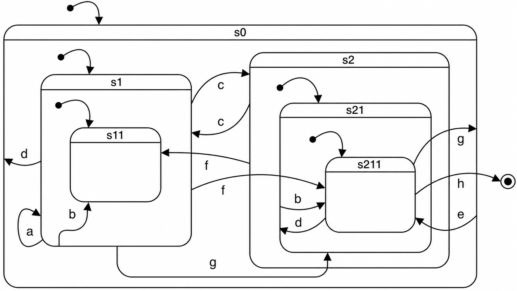
Spaghetti statechart.
The machine starts in s0, follows its initial transition into
s1, and then follows s1's initial transition into
s11. If you send c while the active leaf is
s11, there is no c transition on
s11, so the interpreter looks at the parent
s1 and takes s1 → s2. Entering
s2 then follows nested initial transitions down to
s211.
Spawn the chart and keep the Logger open with the SXML trace filter selected. The trace shows the same process as text: the current configuration, the external event, exits, transitions, and entries.
?- statechart_spawn(Pid, [
       load_uri('/examples/statecharts/02%20spaghetti.xml'),
       trace(true)
   ]).
Use the Examples menu to send events one at a time:
$Pid ! a |
loops on s1 and re-enters its initial leaf s11 |
$Pid ! b |
targets s11 from s1, or s211 from s21 |
$Pid ! c |
moves between the two large sibling regions s1 and s2 |
$Pid ! d |
resets outward to s0, or from s211 to s21 |
$Pid ! e |
uses the outer s0 transition to enter s211 |
$Pid ! f |
crosses between s1, s11, and s211 |
$Pid ! g |
shows leaf-level precedence from s11 or s211 |
$Pid ! h |
takes s211 to final state f and terminates the actor |
NPC emotions
Parallel states let one actor be in several independent states at the same time. This toy non-player character has two emotion dimensions and one behavior mode. At any moment it has one active state in the anger/fear dimension, one in the anticipation/surprise dimension, and one in behavior.
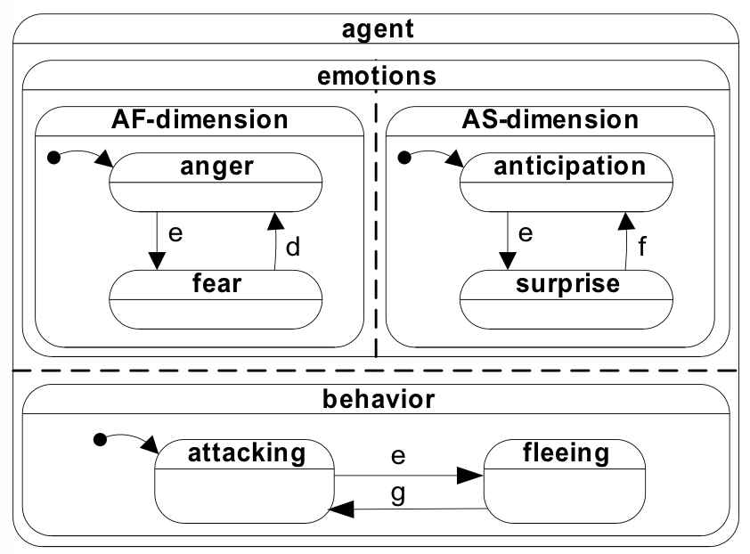
Orthogonal regions: two emotion dimensions plus one behavior mode.
The point of orthogonality is that related but independent dimensions do
not have to be flattened into one large state name. Without parallel
regions, combinations such as anger_anticipation_attacking and
fear_surprise_fleeing would have to be encoded as separate
states, and the number of combinations would grow quickly.
Here, event e can be read as an explosion. Because all three
regions are active, the same event is observed in each region: anger becomes
fear, anticipation becomes surprise, and attacking becomes fleeing in one
coordinated step.
?- statechart_spawn(Pid, [
       load_uri('/examples/statecharts/03%20emotions.xml'),
       trace(true)
   ]).
Use the Examples menu to send the three events:
$Pid ! e |
moves to fear, surprise, and fleeing |
$Pid ! d |
moves fear back to anger and fleeing back to attacking |
$Pid ! f |
moves surprise back to anticipation |
Computing the GCD
The time is ripe to introduce Web Prolog as a scripting language inside statecharts. Executable Web Prolog code in transition bodies and guards increases their power significantly: a chart can update data, run relations, produce output, and still keep the surrounding control logic explicit.
The statechart below applies Euclid's algorithm to find the greatest common
divisor of a list of integers. The machine has two states:
init waits for a single input/1 event carrying
the list, then run iterates — repeatedly replacing
the larger of any two values with their difference — until only
one value remains and the result is printed.
<statechart datamodel="web-prolog" initial="init">
    <datamodel>
        :- dynamic int/1.
    </datamodel>
    <state id="init">
        <go on="input(List)" to="run">
            forall(member(X, List), asserta(int(X)))
        </go>
    </state>
    <state id="run">
        <go if="int(X), int(Y), X > Y">
            Z is X-Y,
            retract(int(X)),
            assert(int(Z))
        </go>
        <go to="stop" if="int(X)">
            writeln(X)
        </go>
    </state>
    <final id="stop" />
</statechart>
Spawn the machine. The Examples menu will be loaded with a sample query:
?- statechart_spawn(Pid, [
       load_uri('/examples/statecharts/08%20gcd.xml'),
       trace(true)
   ]).
Now send the input list:
?- $Pid ! input([25, 10, 15, 30]).
The GCD 5 is computed and written to the terminal, and the
machine has moved to its final state.
A dialogue governor
Statecharts are a good fit for dialogue control: a conversation has
turn-taking, confirmations, repair after misunderstandings, and an
overall flow that is easier to read as a hierarchy of states than as
branching receive/1-2 code. This example is a small
conversational agent that asks the user for the color and size of a
box. Unrecognized input falls back to a history state, which re-enters
the most recently active substate and re-asks its question.
?- statechart_spawn(Pid, [
       load_uri('/examples/statecharts/11%20boxshop-1.xml'),
       trace(true)
   ]).
On entering the color state the machine asks "What color do
you want?". Use the Examples menu to reply. An adjective alone
([red], [blue]) or a full noun phrase
([a, red, box]) parses; anything else triggers the repair
transition.
$Pid ! input([red]). |
parses as color, advances to the size state |
$Pid ! input([a, big, box]). |
parses as size, reaches the final state |
$Pid ! input([hello]). |
does not parse; the agent says "I did not understand" and re-asks the current question |
Three pieces of statechart machinery do the work. First, the
<datamodel> holds a small DCG and two dynamic
predicates (color/1 and size/1) that act as
extracted-fact slots. Second, transitions use
if="phrase(np(color(C)), Input)" to call the DCG as a
guard: the transition only fires when the input parses as the expected
structure, and Prolog variables bound by the parse are in scope in the
transition body. Third, the <history> state and the
outer fallback <go to="h" on="input(Input)"> together
implement local repair: any unparseable input is caught, the agent
apologises, and the history state restores whichever question was
pending, so the conversation continues from where it broke down instead
of restarting.
The whole pattern — explicit states for turn-taking, DCG parsing as a transition guard, and a history-based repair loop — is a compact illustration of why statecharts are well suited to user-facing agents. The same skeleton scales to richer dialogues by adding more states and richer grammars.
Process invocation and communication
Statecharts become more useful once they can spawn other processes and communicate with them. In Web Prolog, the invoked processes are simply actors: toplevels, other statechart actors, or services running on local or remote nodes.
This final example spawns a child toplevel, submits a query to it, prints
each answer as it arrives, and terminates when the last answer has been
received. The spawned toplevel is initialized with a small program:
q(X) :- p(X) and four facts, p(a) through
p(d).
?- statechart_spawn(Pid, [
       load_uri('/examples/statecharts/10%20spawn-toplevel.xml'),
       trace(true)
   ]).
When the surrounding state becomes active, the <spawn>
element creates the child toplevel. The generated
spawned(Pid) event reports the pid of that child actor, and
the transition from ask to collect calls
toplevel_call/3 with limit(1).
<statechart datamodel="web-prolog" initial="spawn-ask-collect">
    <state id="spawn-ask-collect" initial="ask">
        <spawn type="toplevel" exit="false">
            q(X) :- p(X).
            p(a). p(b). p(c). p(d).
        </spawn>
        <state id="ask">
            <go to="collect" on="spawned(Pid)">
                toplevel_call(Pid, q(X), [
                    limit(1)
                ])
            </go>
        </state>
        <state id="collect">
            <go to="collect" on="success(Pid, Data, true)">
                writeln(Data),
                toplevel_next(Pid)
            </go>
            <go to="final" on="success(_, Data, false)">
                writeln(Data)
            </go>
        </state>
    </state>
    <final id="final" />
</statechart>
Each answer arrives as success(Pid, Data, More). While
More is true, the chart prints the current
answer and asks the child toplevel for the next one with
toplevel_next/1. When More is
false, the last answer has arrived and the machine enters its
final state.
Variables bound by the on pattern, and by any
if guard, are in scope in the executable content of the same
<go> element. The intent of <spawn>
is also ownership: the helper process belongs to the control state that
created it, so leaving that state can clean up the invoked actor without
ad hoc shutdown code.
The examples above are just a starting point. More statecharts are available in the Examples drawer; click the arrow to open it and select any file from the Statecharts section. Loading a file opens it in the editor and populates the terminal's Examples menu with its built-in queries, ready to run.
The node's web APIs
Everything so far has used Web Prolog as a programming language — you wrote code, the portal sent it to a node, and the node replied. This closing section looks at the same node from the outside: not as a place to write Prolog, but as a service that other systems can talk to over HTTP and WebSocket. It is the wire-level reference you would consult to embed a Web Prolog node in a JavaScript app, a Python client, or another service.
A Web Prolog node currently exposes three web-facing APIs. The stateless
HTTP API uses /call for self-contained query requests. The
semi-stateful HTTP API uses the /toplevel_* endpoints to keep
a toplevel session alive across several HTTP requests. The stateful
WebSocket API uses /ws for fully interactive, message-based
browser sessions.
The stateless HTTP API
A Web Prolog node can also be queried directly through the stateless
/call endpoint. Because the API is stateless, each request
stands on its own. That makes it easy to try from the browser address
field.
This link runs append([a],[b,c],Xs) and returns JSON:
{{host}}/call?goal=append([a],[b,c],Xs)&format=json
These two links page through the answers to human(Who) on
n4 one slice at a time:
https://n4.elfenbenstornet.se/call?goal=human(Who)&limit=1&offset=0
https://n4.elfenbenstornet.se/call?goal=human(Who)&limit=1&offset=1
In other words, a Web Prolog node can be used both as an interactive Prolog portal and as a simple web API for Prolog queries.
The semi-stateful HTTP API
When one request is not enough, the node also exposes the
/toplevel_spawn, /toplevel_call, and
/toplevel_next endpoints. Together they provide a browser-side
session with paging, output, prompts, and explicit follow-up requests.
Two runnable pages demonstrate the current HTTP session protocol:
-
HTTP demo 1
spawns a toplevel, calls
member(X,[a,b,c])withlimit=1, and fetches the remaining answers one slice at a time. -
HTTP demo 2
loads a session-local program, handles
promptevents, replies withtoplevel_respond, and continues withtoplevel_poll.
The stateful WebSocket API
For fully stateful browser-side interaction, use /ws. The
commands understood by the current node are
toplevel_spawn, toplevel_call,
toplevel_next, toplevel_respond,
spawn, send, and exit.
The following pages are small runnable demonstrations of the current protocol:
-
WebSocket demo 1
queries a toplevel and pages through the answers with
toplevel_next. -
WebSocket demo 2
spawns a browser-owned actor and exchanges messages with the
node-resident
pubsub_service.